---
title: "Results: Ratings"
engine: knitr
execute:
freeze: auto
---
::: {.content-visible when-format="pdf"}
Extended ratings analysis (per-criterion correlations, agreement metrics, human baseline, cost--quality trade-offs) is available in the online supplement at <https://llm-uj-research-eval.netlify.app/results_ratings.html>.
:::
::: {.content-visible when-format="html"}
```{r}
#| label: setup
#| code-summary: "Setup and libraries"
#| code-fold: true
#| message: false
#| warning: false
source("setup_params.R")

library("tidyverse")
library("janitor")
library("stringr")
library("here")
library("knitr")
library("kableExtra")
library("ggrepel")
library("scales")
library("jsonlite")
library("purrr")
library("tibble")
# library("plotly")  # removed: all figures are now static ggplot

# Theme and colors — crisp palette (high saturation, maximum separation)
UJ_ORANGE <- "#E8722A"   # vivid saffron orange
UJ_GREEN  <- "#2D9D5E"   # rich emerald green
UJ_BLUE   <- "#2B7CE9"   # clear azure blue

MODEL_COLORS <- c(
  "GPT-5 Pro"        = "#E8722A",   # saffron orange (focal)
  "GPT-5.2 Pro"      = "#D62839",   # bright crimson
  "GPT-4o-mini"      = "#17B890",   # vivid teal
  "Claude Sonnet 4"  = "#A855F7",   # vivid purple
  "Claude Opus 4.6"  = "#7C3AED",   # deep violet
  "Gemini 2.0 Flash" = "#2B7CE9",   # clear azure
  "Human"            = "#2D9D5E"    # emerald green
)

theme_uj <- function(base_size = 12) {
  theme_minimal(base_size = base_size) +
    theme(
      panel.grid.minor   = element_blank(),
      panel.grid.major   = element_line(linewidth = 0.3, color = "grey88"),
      plot.title          = element_text(face = "bold", size = rel(1.1)),
      plot.title.position = "plot",
      plot.subtitle       = element_text(color = "grey40", size = rel(0.9)),
      plot.caption        = element_text(color = "grey50", size = rel(0.8), hjust = 0),
      axis.title          = element_text(size = rel(0.95)),
      axis.text           = element_text(size = rel(0.88)),
      legend.position     = "bottom",
      legend.text         = element_text(size = rel(0.88)),
      legend.title        = element_text(size = rel(0.9), face = "bold"),
      strip.text          = element_text(face = "bold", size = rel(0.95))
    )
}

canon_metric <- function(x) dplyr::recode(
  x,
  "advancing_knowledge" = "adv_knowledge",
  "open_science"        = "open_sci",
  "logic_communication" = "logic_comms",
  "global_relevance"    = "gp_relevance",
  "claims_evidence"     = "claims",
  .default = x
)

`%||%` <- function(x, y) if (!is.null(x)) x else y

# Pricing per 1M tokens (USD)
pricing <- tribble(
  ~model,              ~input_per_m, ~output_per_m,
  "GPT-5 Pro",         15.00,        60.00,
  "GPT-5.2 Pro",       15.00,        60.00,
  "GPT-4o-mini",       0.15,         0.60,
  "Claude Sonnet 4",   3.00,         15.00,
  "Claude Opus 4.6",   15.00,        75.00,
  "Gemini 2.0 Flash",  0.075,        0.30
)
```
```{r}
#| label: load-human-data
#| code-fold: true
#| code-summary: "Load human evaluation data"
#| message: false
# Load human ratings from Unjournal
UJmap <- read_delim("data/UJ_map.csv", delim = ";", show_col_types = FALSE) |>
  mutate(label_paper_title = research, label_paper = paper) |>
  select(c("label_paper_title", "label_paper"))

rsx <- read_csv("data/rsx_evalr_rating.csv", show_col_types = FALSE) |>
  clean_names() |>
  mutate(label_paper_title = research) |>
  select(-c("research"))

research <- read_csv("data/research.csv", show_col_types = FALSE) |>
  clean_names() |>
  filter(status == "50_published evaluations (on PubPub, by Unjournal)") |>
  left_join(UJmap, by = c("label_paper_title")) |>
  mutate(doi = str_trim(doi)) |>
  mutate(label_paper = case_when(
    doi == "https://doi.org/10.3386/w31162" ~ "Walker et al. 2023",
    doi == "doi.org/10.3386/w32728" ~ "Hahn et al. 2025",
    doi == "https://doi.org/10.3386/w30011" ~ "Bhat et al. 2022",
    doi == "10.1093/wbro/lkae010" ~ "Crawfurd et al. 2023",
    TRUE ~ label_paper
  )) |>
  left_join(rsx, by = c("label_paper_title"))

key_map <- research |>
  transmute(label_paper_title = str_trim(label_paper_title), label_paper = label_paper) |>
  filter(!is.na(label_paper_title)) |>
  distinct(label_paper_title, label_paper) |>
  group_by(label_paper_title) |>
  slice(1) |>
  ungroup()

rsx_research <- rsx |>
  mutate(label_paper_title = str_trim(label_paper_title)) |>
  left_join(key_map, by = "label_paper_title", relationship = "many-to-one")

metrics_human <- rsx_research |>
  mutate(criteria = canon_metric(criteria)) |>
  filter(criteria %in% c("overall", "claims", "methods", "adv_knowledge", "logic_comms", "open_sci", "gp_relevance")) |>
  transmute(
    paper = label_paper, criteria, evaluator, model = "Human",
    mid = as.numeric(middle_rating),
    lo = suppressWarnings(as.numeric(lower_ci)),
    hi = suppressWarnings(as.numeric(upper_ci))
  ) |>
  filter(!is.na(paper), !is.na(mid)) |>
  mutate(
    lo = ifelse(is.finite(lo), pmax(0, pmin(100, lo)), NA_real_),
    hi = ifelse(is.finite(hi), pmax(0, pmin(100, hi)), NA_real_)
  ) |>
  mutate(across(c(mid, lo, hi), ~ round(.x, 4))) |>
  distinct(paper, criteria, model, evaluator, mid, lo, hi)

human_avg <- metrics_human |>
  filter(criteria == "overall") |>
  group_by(paper) |>
  summarise(
    human_mid = mean(mid, na.rm = TRUE),
    human_lo = mean(lo, na.rm = TRUE),
    human_hi = mean(hi, na.rm = TRUE),
    n_human = n(),
    .groups = "drop"
  )

# Summary stats for inline use
n_human_papers <- n_distinct(metrics_human$paper)
n_human_evaluators <- n_distinct(metrics_human$evaluator)
```
```{r}
#| label: load-llm-data
#| code-fold: true
#| code-summary: "Load LLM evaluation data (all models)"
#| message: false
model_dirs <- list(
  "gpt5_pro_updated_jan2026" = "GPT-5 Pro",
  "gpt52_pro_focal_jan2026" = "GPT-5.2 Pro",
  "gpt_4o_mini_2024_07_18" = "GPT-4o-mini",
  "claude_sonnet_4_20250514" = "Claude Sonnet 4",
  "claude_opus_4_6" = "Claude Opus 4.6",
  "gemini_2.0_flash" = "Gemini 2.0 Flash"
)

parse_response <- function(path, model_name) {
  tryCatch({
    r <- jsonlite::fromJSON(path, simplifyVector = FALSE)
    paper <- basename(path) |>
      str_replace("\\.response\\.json$", "") |>
      str_replace_all("_", " ")

    parsed <- NULL
    if (!is.null(r$parsed) && length(r$parsed) > 0) {
      parsed <- r$parsed
    } else if (!is.null(r$output_text) && nchar(r$output_text) > 0) {
      # Strip markdown code fences if present
      txt <- r$output_text
      txt <- sub("^\\s*```[a-z]*\\s*\n?", "", txt)
      txt <- sub("\\s*```\\s*$", "", txt)
      parsed <- jsonlite::fromJSON(txt, simplifyVector = TRUE)
    } else if (!is.null(r$output)) {
      msg <- purrr::detect(r$output, ~ .x$type == "message", .default = NULL)
      if (!is.null(msg) && length(msg$content) > 0) {
        parsed <- jsonlite::fromJSON(msg$content[[1]]$text, simplifyVector = TRUE)
      }
    }

    if (is.null(parsed)) return(NULL)

    metrics <- parsed$metrics
    metric_rows <- list()
    tier_rows <- list()

    tier_names <- c("tier_should", "tier_will", "journal_should", "journal_will")

    for (nm in names(metrics)) {
      if (nm %in% tier_names) {
        # Normalise journal_should/journal_will → tier_should/tier_will
        tier_kind <- sub("^journal_", "tier_", nm)
        tier_rows[[length(tier_rows) + 1]] <- tibble(
          paper = paper, model = model_name, tier_kind = tier_kind,
          score = metrics[[nm]]$score,
          ci_lower = metrics[[nm]]$ci_lower,
          ci_upper = metrics[[nm]]$ci_upper
        )
      } else {
        metric_rows[[length(metric_rows) + 1]] <- tibble(
          paper = paper, model = model_name, metric = nm,
          midpoint = metrics[[nm]]$midpoint,
          lower_bound = metrics[[nm]]$lower_bound,
          upper_bound = metrics[[nm]]$upper_bound
        )
      }
    }

    input_tok <- r$usage$input_tokens %||% r$input_tokens
    output_tok <- r$usage$output_tokens %||% r$output_tokens
    reasoning_tok <- r$usage$output_tokens_details$reasoning_tokens

    list(
      metrics = bind_rows(metric_rows),
      tiers = bind_rows(tier_rows),
      tokens = tibble(
        paper = paper, model = model_name,
        input_tokens = input_tok %||% NA_integer_,
        output_tokens = output_tok %||% NA_integer_,
        reasoning_tokens = reasoning_tok %||% NA_integer_
      ),
      summary = tibble(
        paper = paper, model = model_name,
        assessment_summary = parsed$assessment_summary
      )
    )
  }, error = function(e) NULL)
}

load_all_llm <- function() {
  all_metrics <- list()
  all_tiers <- list()
  all_tokens <- list()
  all_summaries <- list()

  for (dir_name in names(model_dirs)) {
    model_name <- model_dirs[[dir_name]]
    json_dir <- here("results", dir_name, "json")

    if (dir.exists(json_dir)) {
      files <- list.files(json_dir, pattern = "\\.response\\.json$", full.names = TRUE)

      for (f in files) {
        result <- parse_response(f, model_name)
        if (!is.null(result)) {
          all_metrics[[length(all_metrics) + 1]] <- result$metrics
          all_tiers[[length(all_tiers) + 1]] <- result$tiers
          all_tokens[[length(all_tokens) + 1]] <- result$tokens
          all_summaries[[length(all_summaries) + 1]] <- result$summary
        }
      }
    }
  }

  list(
    metrics = bind_rows(all_metrics) |> mutate(criteria = canon_metric(metric)),
    tiers = bind_rows(all_tiers),
    tokens = bind_rows(all_tokens),
    summaries = bind_rows(all_summaries)
  )
}

llm_data <- load_all_llm()
llm_metrics <- llm_data$metrics
llm_tiers <- llm_data$tiers
llm_tokens <- llm_data$tokens
llm_summaries <- llm_data$summaries

# Reconcile LLM filenames with human labels where the citation year differs but
# the manuscript is the same (verified by title/DOI/content). See results.qmd.
canon_paper <- function(x) dplyr::recode(
  x,
  "Trammel and Aschenbrenner 2024" = "Trammel and Aschenbrenner 2025",
  "Liang et al 2023"               = "Liang et al. 2021",
  .default = x
)
llm_metrics   <- llm_metrics   |> mutate(paper = canon_paper(paper))
llm_tiers     <- llm_tiers     |> mutate(paper = canon_paper(paper))
llm_tokens    <- llm_tokens    |> mutate(paper = canon_paper(paper))
if (!is.null(llm_summaries) && nrow(llm_summaries) > 0) {
  llm_summaries <- llm_summaries |> mutate(paper = canon_paper(paper))
}

# Summary stats for inline use
n_llm_models <- n_distinct(llm_metrics$model)
n_llm_papers <- n_distinct(llm_metrics$paper)
llm_model_names <- unique(llm_metrics$model)
llm_model_list <- paste(llm_model_names, collapse = ", ")

# Papers with both human and LLM data
matched_papers <- intersect(
 unique(metrics_human$paper),
 unique(llm_metrics$paper)
)
n_matched <- length(matched_papers)

# Opus sample: papers evaluated by Claude Opus 4.6 AND humans
# Agreement tables and Krippendorff alpha use this sample so all
# models are compared on the same set of papers.
opus_papers <- intersect(
  llm_metrics |> filter(model == "Claude Opus 4.6") |> pull(paper) |> unique(),
  unique(metrics_human$paper)
)
n_opus <- length(opus_papers)

# Cost summary
cost_data <- llm_tokens |>
  left_join(pricing, by = "model") |>
  mutate(
    reasoning_tokens = coalesce(reasoning_tokens, 0L),
    cost_usd = (input_tokens * input_per_m + output_tokens * output_per_m) / 1e6
  )

total_cost <- sum(cost_data$cost_usd, na.rm = TRUE)
total_evaluations <- nrow(llm_tokens)

# Per-model summaries
model_summary <- cost_data |>
  group_by(model) |>
  summarise(
    n_papers = n(),
    avg_input = round(mean(input_tokens, na.rm = TRUE)),
    avg_output = round(mean(output_tokens, na.rm = TRUE)),
    avg_reasoning = round(mean(reasoning_tokens[reasoning_tokens > 0], na.rm = TRUE)),
    total_cost = sum(cost_usd, na.rm = TRUE),
    cost_per_paper = mean(cost_usd, na.rm = TRUE),
    .groups = "drop"
  )
```
We compare quantitative ratings from `r n_llm_models` frontier LLMs (`r llm_model_list`) against human expert reviews from [The Unjournal](https://unjournal.pubpub.org). Across all models, `r n_matched` papers have both human and LLM evaluations. Agreement metrics and Krippendorff's alpha below are computed on the `r n_opus`-paper matched sample with Claude Opus 4.6 evaluations, so that all models are compared on identical papers.
We submit each PDF through a single, schema-enforced API call. The system prompt mirrors The Unjournal rubric, blocks extrinsic priors (authors, venue, web context), and requires strict JSON: a ~1k-word diagnostic summary plus numeric midpoints and 90% credible intervals for every metric.^[0–100 percentiles relative to a reference group of ~'all serious work you have read in this area in the last three years', overall (global quality/impact), claims_evidence (claim clarity/support), methods (design/identification/robustness), advancing_knowledge (contribution to field/practice), logic_communication (internal consistency and exposition), open_science (reproducibility, data/code availability), and global_relevance (decision and priority usefulness). Journal tiers: (0–5, continuous) capture where the work should publish vs. will publish.] Each numeric field carries a midpoint (model's 50% belief) and a 90% credible interval; wide intervals indicate acknowledged uncertainty.
**Cost and token usage.** Token costs are computed from API-reported input/output tokens (GPT-5 Pro runs with `reasoning` = high).
```{r}
#| label: tbl-cost-overview
#| tbl-cap: "Token usage and estimated cost per model"
if (nrow(llm_tokens) > 0) {

  cost_table <- model_summary |>
    transmute(
      Model = model,
      Papers = n_papers,
      `Avg input` = scales::comma(avg_input),
      `Avg output` = scales::comma(avg_output),
      `Avg reasoning` = ifelse(is.finite(avg_reasoning) & avg_reasoning > 0,
                                scales::comma(avg_reasoning), "—"),
      `Total cost` = scales::dollar(total_cost, accuracy = 0.01),
      `Cost/paper` = scales::dollar(cost_per_paper, accuracy = 0.001)
    ) |>
    arrange(desc(as.numeric(gsub("[$,]", "", `Total cost`))))

  knitr::kable(cost_table, align = c("l", rep("r", 6)))
}
```
Total cost across all `r total_evaluations` LLM evaluations: **`r scales::dollar(total_cost, accuracy = 0.01)`**. Reasoning-capable models (GPT-5 Pro, GPT-5.2 Pro, Claude Opus 4.6) cost substantially more per paper than their lighter counterparts (GPT-4o-mini, Gemini 2.0 Flash), raising practical questions about cost-quality trade-offs for deployment at scale.
```{r}
#| label: scatter-data-prep
#| include: false
# Prepare scatter_data for tbl-agreement — restricted to common sample
scatter_data <- llm_metrics |>
filter(criteria == "overall", paper %in% opus_papers) |>
inner_join(human_avg, by = "paper") |>
mutate(
diff = midpoint - human_mid,
paper_short = str_trunc(paper, 25),
human_lo = coalesce(human_lo, human_mid),
human_hi = coalesce(human_hi, human_mid),
lower_bound = coalesce(lower_bound, midpoint),
upper_bound = coalesce(upper_bound, midpoint)
) |>
filter(!is.na(human_mid), !is.na(midpoint))
```
```{r}
#| label: compute-hh-baseline
#| include: false
# Human-Human pairwise agreement (baseline for agreement tables).
# For papers with ≥2 evaluators, assign E1/E2 by row order within paper,
# then compute pairwise correlation and error metrics across all such papers.
hh_pairs <- metrics_human |>
filter(criteria == "overall", paper %in% opus_papers) |>
select(paper, evaluator, mid) |>
distinct() |>
group_by(paper) |>
filter(n() >= 2) |>
mutate(slot = paste0("E", row_number())) |>
ungroup() |>
pivot_wider(names_from = slot, values_from = c(mid, evaluator)) |>
filter(!is.na(mid_E1), !is.na(mid_E2))
hh_n <- nrow(hh_pairs)
hh_pearson <- round(cor(hh_pairs$mid_E1, hh_pairs$mid_E2), 3)
hh_spearman <- round(cor(hh_pairs$mid_E1, hh_pairs$mid_E2, method = "spearman"), 3)
hh_mae <- round(mean(abs(hh_pairs$mid_E1 - hh_pairs$mid_E2), na.rm = TRUE), 1)
hh_rmse <- round(sqrt(mean((hh_pairs$mid_E1 - hh_pairs$mid_E2)^2, na.rm = TRUE)), 1)
hh_bias <- sprintf("%+.1f", mean(hh_pairs$mid_E1 - hh_pairs$mid_E2, na.rm = TRUE))
hh_baseline_row <- tibble(
Model = "Human\u2013Human",
N = hh_n,
`Spearman ρ` = hh_spearman,
`Pearson r` = hh_pearson,
`Mean bias` = hh_bias,
RMSE = hh_rmse,
MAE = hh_mae
)
# Spearman-Brown correction factor.
# LLM rho is computed against the k-rater human mean (smoother signal) while
# rho_HH compares individual raters. Multiply raw rho_HL by sb_factor to
# convert to the individual-rater-equivalent scale for a fair comparison.
k_raters <- metrics_human |>
filter(criteria == "overall", paper %in% opus_papers) |>
group_by(paper) |>
summarise(k = n_distinct(evaluator), .groups = "drop") |>
summarise(k = mean(k)) |>
pull(k)
r_kk <- k_raters * hh_spearman / (1 + (k_raters - 1) * hh_spearman)
sb_factor <- sqrt(hh_spearman / r_kk)
# Fisher-z 95% CI for Spearman rho
spearman_ci95 <- function(rho, n) {
if (is.na(rho) || n < 4) return("—")
z <- atanh(rho)
se <- 1 / sqrt(n - 3)
sprintf("[%.2f, %.2f]", tanh(z - 1.96 * se), tanh(z + 1.96 * se))
}
```
**Agreement metrics.** We report Spearman *ρ*, MAE, mean bias, and Pearson *r*. The **H–H row** shows individual-vs-individual *ρ* — it is already on the natural scale and serves as the reference. **LLM rows** show *ρ* against the human *mean* rating (of `r round(k_raters, 1)` raters/paper), which is upward-biased relative to H–H because averaging suppresses noise. The **ρ adj.** column applies the Spearman-Brown correction to LLM rows only (×`r sprintf("%.2f", sb_factor)`), converting them to the individual-rater-equivalent scale so they are directly comparable to the H–H *ρ*.
```{r}
#| label: tbl-agreement
#| tbl-cap: "Agreement between each LLM and human mean overall rating, matched sample (N = `r n_opus`). **Spearman ρ column**: for the H–H row this is individual-vs-individual ρ (the reference, already on the natural scale); for LLM rows it is ρ vs. the human *mean* (upward-biased because the mean is smoother than any individual rater). **ρ adj.**: Spearman-Brown corrected to individual-rater-equivalent scale (×`r sprintf('%.2f', sb_factor)` for k≈`r round(k_raters, 1)` raters/paper) — apply this correction to compare LLM rows fairly to H–H. H–H shows — in the ρ adj. column because no correction is needed. **95% CI**: Fisher-z. Bias = LLM − Human. †N < 15: unreliable."
MIN_N <- 15

if (nrow(scatter_data) > 0) {

  # Helper: summarise one data frame into a table row per model
  model_agreement_rows <- function(df) {
    df |>
      group_by(Model = model) |>
      summarise(
        N           = n(),
        raw_rho     = cor(human_mid, midpoint, method = "spearman", use = "complete.obs"),
        `Pearson r` = round(cor(human_mid, midpoint, use = "complete.obs"), 3),
        `Mean bias` = sprintf("%+.1f", mean(midpoint - human_mid, na.rm = TRUE)),
        MAE         = sprintf("%.1f", mean(abs(midpoint - human_mid), na.rm = TRUE)),
        .groups     = "drop"
      ) |>
      arrange(desc(raw_rho)) |>
      mutate(
        flag           = ifelse(N < MIN_N, "†", ""),
        `Spearman ρ` = sprintf("%.3f%s", raw_rho, flag),
        `ρ adj.`  = sprintf("%.3f%s", raw_rho * sb_factor, flag),
        `95% CI`       = mapply(spearman_ci95, raw_rho, N)
      ) |>
      select(Model, N, `Spearman ρ`, `ρ adj.`, `95% CI`,
             `Pearson r`, `Mean bias`, MAE)
  }

  # Matched sample: only papers where H-H comparison is also available (≥2 human raters)
  lfl_set     <- hh_pairs$paper
  llm_matched <- model_agreement_rows(scatter_data |> filter(paper %in% lfl_set))
  llm_full    <- model_agreement_rows(scatter_data)

  hh_row <- tibble(
    Model          = "Human–Human",
    N              = hh_n,
    `Spearman ρ` = sprintf("%.3f", hh_spearman),
    `ρ adj.`  = "—",
    `95% CI`       = spearman_ci95(hh_spearman, hh_n),
    `Pearson r`    = round(hh_pearson, 3),
    `Mean bias`    = hh_bias,
    MAE            = sprintf("%.1f", hh_mae)
  )

  n_matched <- nrow(llm_matched)
  n_full    <- nrow(llm_full)

  agreement_tbl <- bind_rows(hh_row, llm_matched, llm_full)

  knitr::kable(agreement_tbl, align = c("l", rep("r", ncol(agreement_tbl) - 1))) |>
    kableExtra::row_spec(1, bold = TRUE, background = "#f0f8f0") |>
    kableExtra::pack_rows(
      sprintf("Matched sample — same %d papers as H–H baseline (primary comparison)", hh_n),
      1, 1 + n_matched, bold = TRUE, italic = FALSE, color = "black"
    ) |>
    kableExtra::pack_rows(
      sprintf("Full opus sample — each model's own N (up to %d; secondary)", n_opus),
      2 + n_matched, 1 + n_matched + n_full, bold = FALSE, italic = TRUE
    )
}
```
@tbl-agreement is organised in two groups. The **primary matched-sample group** restricts both the H–H baseline and all LLM rows to the same `r hh_n` papers that have ≥2 human raters — this is the only fair like-for-like comparison (same denominator for every row). The **secondary full-sample group** uses each model's own maximum N (up to `r n_opus`), which increases power at the cost of cross-row comparability. **Spearman ρ** is upward-biased relative to ρ_HH because LLMs are evaluated against the mean of `r round(k_raters, 1)` human raters; **ρ adj.** applies the Spearman-Brown correction (×`r sprintf("%.2f", sb_factor)`) for a fair comparison to the H–H *ρ* of `r hh_spearman`. 95% CIs (Fisher-z) are wide at these sample sizes. Models with N < 15 (†) are unreliable.
@tbl-agreement-full repeats the same structure using each model's own maximum matched sample.
```{r}
#| label: tbl-agreement-full
#| tbl-cap: "Agreement between each LLM and human mean overall rating, using each model's own maximum matched sample (not restricted to the common `r n_opus`-paper set). Larger N per model but cross-model comparison is confounded by paper-set differences. Same column structure as @tbl-agreement: H–H Spearman *ρ* is individual-vs-individual; LLM Spearman *ρ* is vs. human mean (upward-biased); ρ adj. is Spearman-Brown corrected for fair comparison."
if (nrow(llm_metrics) > 0 && nrow(human_avg) > 0) {

  scatter_full <- llm_metrics |>
    filter(criteria == "overall") |>
    inner_join(human_avg |> select(paper, human_mid), by = "paper") |>
    filter(!is.na(human_mid), !is.na(midpoint))

  # HH baseline on all matched papers (not restricted to opus_papers)
  hh_pairs_full <- metrics_human |>
    filter(criteria == "overall", paper %in% unique(scatter_full$paper)) |>
    select(paper, evaluator, mid) |>
    distinct() |>
    group_by(paper) |>
    filter(n() >= 2) |>
    mutate(slot = paste0("E", row_number())) |>
    ungroup() |>
    pivot_wider(names_from = slot, values_from = c(mid, evaluator)) |>
    filter(!is.na(mid_E1), !is.na(mid_E2))

  hh_rho_full <- round(cor(hh_pairs_full$mid_E1, hh_pairs_full$mid_E2,
                             method = "spearman"), 3)

  k_full <- metrics_human |>
    filter(criteria == "overall", paper %in% unique(scatter_full$paper)) |>
    group_by(paper) |>
    summarise(k = n_distinct(evaluator), .groups = "drop") |>
    summarise(k = mean(k)) |>
    pull(k)
  r_kk_full  <- k_full * hh_rho_full / (1 + (k_full - 1) * hh_rho_full)
  sb_full    <- sqrt(hh_rho_full / r_kk_full)

  lfl_set_full <- hh_pairs_full$paper  # papers with >=2 human raters in full matched set

  model_agreement_rows_full <- function(df) {
    df |>
      group_by(Model = model) |>
      summarise(
        N           = n(),
        raw_rho     = cor(human_mid, midpoint, method = "spearman", use = "complete.obs"),
        `Pearson r` = round(cor(human_mid, midpoint, use = "complete.obs"), 3),
        `Mean bias` = sprintf("%+.1f", mean(midpoint - human_mid, na.rm = TRUE)),
        MAE         = sprintf("%.1f", mean(abs(midpoint - human_mid), na.rm = TRUE)),
        .groups     = "drop"
      ) |>
      arrange(desc(raw_rho)) |>
      mutate(
        flag           = ifelse(N < 15, "†", ""),
        `Spearman ρ` = sprintf("%.3f%s", raw_rho, flag),
        `ρ adj.`  = sprintf("%.3f%s", raw_rho * sb_full, flag),
        `95% CI`       = mapply(spearman_ci95, raw_rho, N)
      ) |>
      select(Model, N, `Spearman ρ`, `ρ adj.`, `95% CI`,
             `Pearson r`, `Mean bias`, MAE)
  }

  llm_matched_full <- model_agreement_rows_full(scatter_full |> filter(paper %in% lfl_set_full))
  llm_all_full     <- model_agreement_rows_full(scatter_full)

  hh_row_full <- tibble(
    Model               = "Human–Human",
    N                   = nrow(hh_pairs_full),
    `Spearman ρ` = sprintf("%.3f", hh_rho_full),
    `ρ adj.`  = "—",
    `95% CI`            = spearman_ci95(hh_rho_full, nrow(hh_pairs_full)),
    `Pearson r`         = round(cor(hh_pairs_full$mid_E1, hh_pairs_full$mid_E2), 3),
    `Mean bias`         = "—",
    MAE                 = "—"
  )

  n_mf <- nrow(llm_matched_full)
  n_af <- nrow(llm_all_full)

  tbl_full <- bind_rows(hh_row_full, llm_matched_full, llm_all_full)

  knitr::kable(tbl_full, align = c("l", rep("r", ncol(tbl_full) - 1))) |>
    kableExtra::row_spec(1, bold = TRUE, background = "#f0f8f0") |>
    kableExtra::pack_rows(
      sprintf("Matched sample — same %d papers as H–H baseline (primary)", nrow(hh_pairs_full)),
      1, 1 + n_mf, bold = TRUE, italic = FALSE, color = "black"
    ) |>
    kableExtra::pack_rows(
      "Full per-model sample — each model's own maximum N (secondary)",
      2 + n_mf, 1 + n_mf + n_af, bold = FALSE, italic = TRUE
    ) |>
    kableExtra::footnote(symbol = "† N < 15 papers; estimates unreliable.")
}
```
**Human baseline context.** Human percentile ratings are a noisy reference signal, not ground truth: even expert evaluators given the same paper differ systematically, reflecting genuine uncertainty in what a "correct" score would be. @tbl-human-baseline quantifies this noise as Krippendorff's α~HH~. The α~HL~ columns show how close each LLM comes to that level. A model with α~HL~ ≈ α~HH~ on a criterion is generating signal comparable to a second human evaluator on that dimension. Criteria where α~HH~ is already low indicate genuine expert disagreement; low α~HL~ on those criteria is therefore expected, not a model failure.
```{r}
#| label: tbl-human-baseline
#| tbl-cap: "Krippendorff's α~HH~ (agreement within the human-evaluator panel) vs α~HL~ (agreement when the LLM is added to that panel) by criterion. Both are computed on the same papers and use individual human rater scores—not the human mean—so the comparison is symmetric. If α~HL~ ≈ α~HH~, the LLM behaves like an additional human evaluator on that criterion. Column headers show N papers per model; models with N < 15 (marked †) are unreliable."
#| code-fold: true
if (requireNamespace("irr", quietly = TRUE)) {

  library(irr)

  criteria_list <- c("overall", "claims", "methods", "adv_knowledge",
                     "logic_comms", "open_sci", "gp_relevance")

  criterion_labels <- c(
    overall = "Overall", claims = "Claims", methods = "Methods",
    adv_knowledge = "Adv. Knowledge", logic_comms = "Logic & Comms",
    open_sci = "Open Science", gp_relevance = "Global Relevance"
  )

  # Compute human-human alpha (each evaluator as separate rater)
  compute_hh_alpha <- function(criterion) {
    human_wide <- metrics_human |>
      filter(criteria == criterion, paper %in% opus_papers) |>
      select(paper, evaluator, mid) |>
      distinct() |>
      pivot_wider(names_from = paper, values_from = mid)

    if (nrow(human_wide) < 2 || ncol(human_wide) < 3) return(NA_real_)

    M <- as.matrix(human_wide[, -1, drop = FALSE])
    tryCatch({
      irr::kripp.alpha(M, method = "interval")$value
    }, error = function(e) NA_real_)
  }

  # Compute human-LLM alpha using full panel [H1, H2, ..., LLM].
  # Adding LLM as an additional rater alongside individual humans (not the mean)
  # removes the mean-vs-individual bias and answers: does the LLM behave like
  # an additional human evaluator on this criterion?
  compute_hl_alpha <- function(criterion, model_name) {
    # Individual human ratings: rows = evaluators, cols = papers
    human_wide <- metrics_human |>
      filter(criteria == criterion, paper %in% opus_papers) |>
      select(paper, evaluator, mid) |>
      distinct() |>
      pivot_wider(names_from = paper, values_from = mid)

    if (nrow(human_wide) < 2 || ncol(human_wide) < 3) return(NA_real_)
    M_human <- as.matrix(human_wide[, -1, drop = FALSE])

    # LLM ratings as a named vector over the same papers
    llm_vals <- llm_metrics |>
      filter(criteria == criterion, model == model_name, paper %in% opus_papers) |>
      select(paper, midpoint) |>
      distinct()

    if (nrow(llm_vals) < 3) return(NA_real_)

    # Build LLM row aligned to same paper columns as M_human
    llm_row <- matrix(NA_real_, nrow = 1, ncol = ncol(M_human))
    colnames(llm_row) <- colnames(M_human)
    common <- intersect(colnames(M_human), llm_vals$paper)
    if (length(common) < 3) return(NA_real_)
    llm_row[1, common] <- llm_vals$midpoint[match(common, llm_vals$paper)]

    # Panel: all individual human raters + LLM as one additional rater
    M <- rbind(M_human, llm_row)
    tryCatch({
      irr::kripp.alpha(M, method = "interval")$value
    }, error = function(e) NA_real_)
  }

  # Get unique LLM models and their paper counts (to flag low-N columns)
  llm_models <- unique(llm_metrics$model)
  model_n_df <- llm_metrics |>
    filter(criteria == "overall", paper %in% opus_papers) |>
    group_by(model) |>
    summarise(n = n_distinct(paper), .groups = "drop")
  model_n_map <- setNames(model_n_df$n, model_n_df$model)

  MIN_N_ALPHA <- 15

  # Build comparison table
  baseline_results <- tibble(Criterion = criterion_labels[criteria_list]) |>
    mutate(criterion_key = criteria_list) |>
    rowwise() |>
    mutate(
      `α_HH` = compute_hh_alpha(criterion_key)
    ) |>
    ungroup()

  # Add columns for each LLM model, labelled with N and flagged if N < MIN_N_ALPHA
  for (mod in llm_models) {
    n_mod        <- if (mod %in% names(model_n_map)) as.integer(model_n_map[mod]) else 0L
    n_label      <- if (n_mod < MIN_N_ALPHA) sprintf("n=%d†", n_mod) else sprintf("n=%d", n_mod)
    col_raw      <- paste0("α_HL (", mod, ")")
    col_labelled <- paste0("α_HL ", mod, " (", n_label, ")")
    baseline_results <- baseline_results |>
      rowwise() |>
      mutate(!!col_raw := compute_hl_alpha(criterion_key, mod)) |>
      ungroup()
    names(baseline_results)[names(baseline_results) == col_raw] <- col_labelled
  }

  # Format for display — put α_HH immediately after Criterion column
  baseline_display <- baseline_results |>
    select(-criterion_key) |>
    mutate(across(where(is.numeric), ~ ifelse(is.na(.x), "\u2014", sprintf("%.2f", .x))))

  alpha_col_order <- c("Criterion", "\u03b1_HH",
                       sort(grep("^\u03b1_HL", names(baseline_display), value = TRUE)))
  existing_cols <- alpha_col_order[alpha_col_order %in% names(baseline_display)]
  baseline_display <- baseline_display |> select(all_of(existing_cols))

  knitr::kable(baseline_display, align = c("l", rep("r", ncol(baseline_display) - 1))) |>
    kableExtra::column_spec(2, bold = TRUE) |>
    kableExtra::footnote(
      symbol = "\u2020 N < 15 papers; \u03b1_HL unreliable for this model."
    )
}
```
Both α~HH~ and α~HL~ are computed on the same individual human-rater scores—not the human mean—making the comparison symmetric: α~HL~ asks whether adding the LLM to the human panel maintains the same level of agreement as the humans achieve among themselves. Where α~HL~ ≈ α~HH~, the LLM is behaving like an additional human evaluator. Criteria where α~HH~ is already low indicate genuine evaluator disagreement; low α~HL~ there reflects task difficulty rather than a model failure.
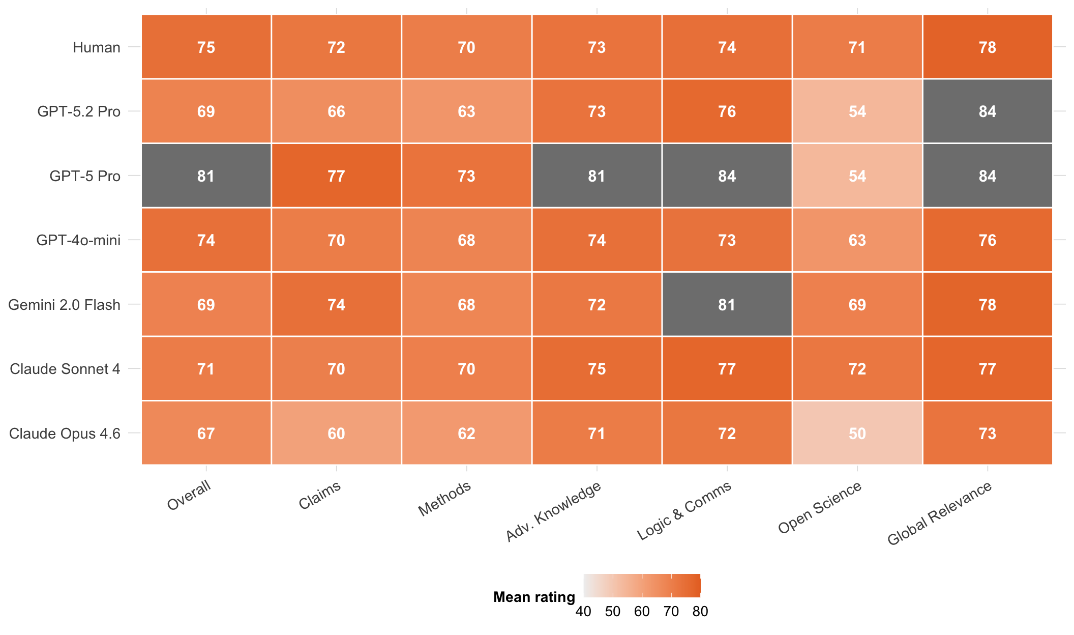
**Criteria-level patterns.** @fig-criteria-heatmap displays the mean rating each evaluator type assigns across the seven criteria. Criteria where all models and humans converge (similar colour intensity) suggest robust agreement on that dimension; criteria with divergent columns indicate systematic differences in how humans and LLMs weigh that aspect of quality.
```{r}
#| label: fig-criteria-heatmap
#| fig-cap: "Mean rating by evaluator type (rows) and criterion (columns), averaged across all matched papers. Tile colour scales from light (lower mean) to vivid orange (higher mean), clamped to 40\u201380. Criteria where all rows show similar colour intensity indicate broad agreement; divergent columns flag criteria-level systematic differences."
#| fig-width: 11
#| fig-height: 6.5
metric_labels <- c(
  overall = "Overall", claims = "Claims", methods = "Methods",
  adv_knowledge = "Adv. Knowledge", logic_comms = "Logic & Comms",
  open_sci = "Open Science", gp_relevance = "Global Relevance"
)

criteria_means <- bind_rows(
  metrics_human |>
    filter(criteria %in% names(metric_labels), paper %in% matched_papers) |>
    group_by(criteria) |>
    summarise(mean_rating = mean(mid, na.rm = TRUE), .groups = "drop") |>
    mutate(model = "Human"),
  llm_metrics |>
    filter(criteria %in% names(metric_labels), paper %in% matched_papers) |>
    group_by(model, criteria) |>
    summarise(mean_rating = mean(midpoint, na.rm = TRUE), .groups = "drop")
) |>
  mutate(criteria_label = factor(metric_labels[criteria], levels = metric_labels))

if (nrow(criteria_means) > 0) {
  ggplot(criteria_means, aes(x = criteria_label, y = model, fill = mean_rating)) +
    geom_tile(color = "white", linewidth = 0.5) +
    geom_text(aes(label = round(mean_rating, 0)), size = 4.2, color = "white", fontface = "bold") +
    scale_fill_gradient(low = "#f0f0f0", high = UJ_ORANGE, limits = c(40, 80), name = "Mean rating") +
    labs(x = NULL, y = NULL) +
    theme_uj() +
    theme(axis.text.x = element_text(angle = 30, hjust = 1, size = 11),
          axis.text.y = element_text(size = 11),
          panel.grid = element_blank())
}
```
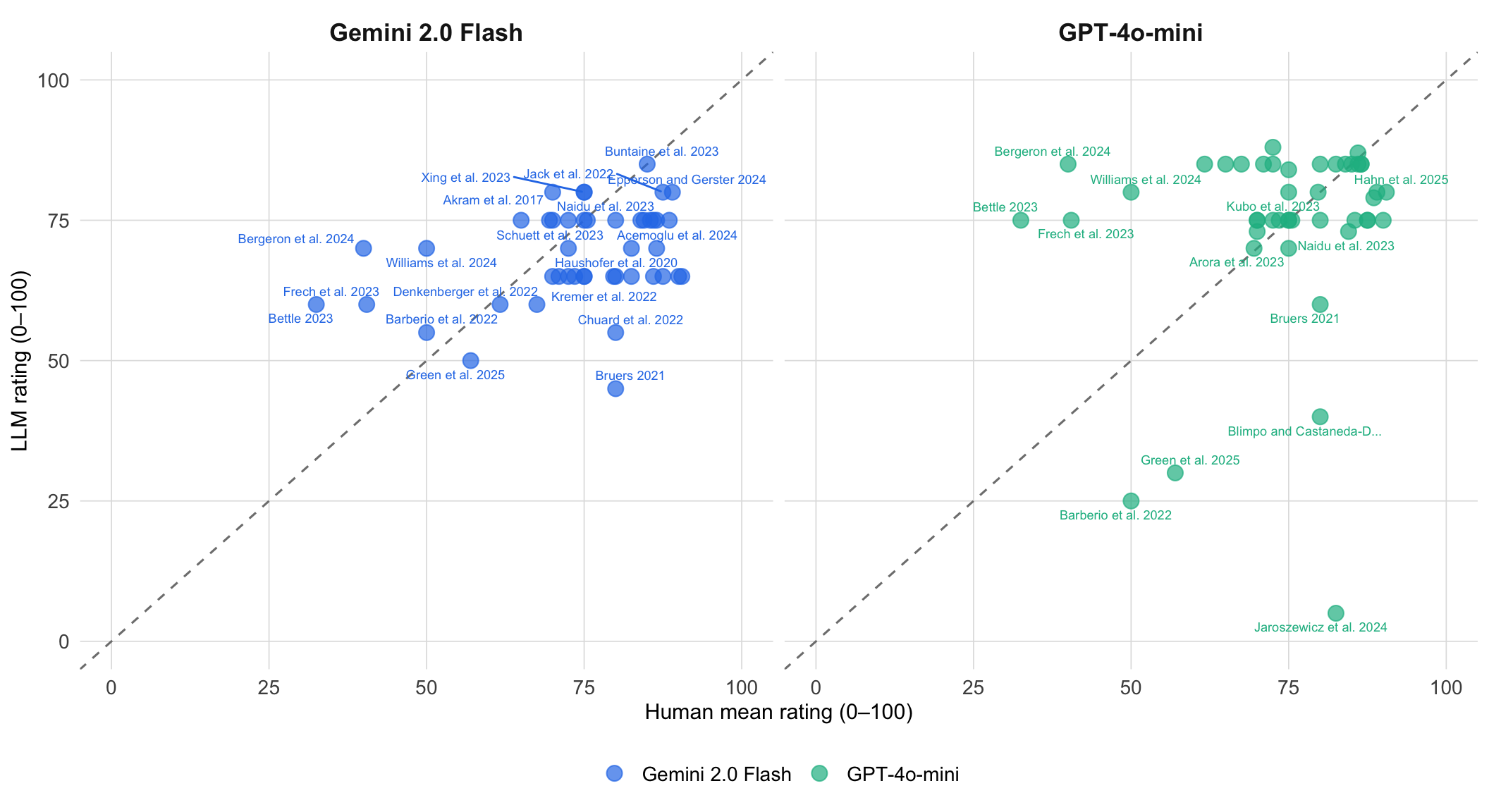
**Additional models.** @fig-scatter-other shows overall ratings for the two lightweight models---GPT-4o-mini and Gemini 2.0 Flash---against human mean ratings. These models cost 50--200× less per paper than reasoning-capable models (see @tbl-cost-overview) but may sacrifice rating accuracy.
```{r}
#| label: fig-scatter-other
#| fig-cap: "Human mean overall rating (x-axis) vs LLM overall rating (y-axis) for the two lightweight models GPT-4o-mini and Gemini 2.0 Flash. Each point is one paper; the dashed diagonal is the identity line. These models cost 50\u2013200\u00d7 less per paper than reasoning-capable models (see cost table above)."
#| fig-width: 11
#| fig-height: 6
other_models <- c("GPT-4o-mini", "Gemini 2.0 Flash")

scatter_other <- llm_metrics |>
  filter(criteria == "overall", model %in% other_models) |>
  inner_join(human_avg, by = "paper") |>
  mutate(
    diff = midpoint - human_mid,
    paper_short = str_trunc(paper, 25),
    human_lo = coalesce(human_lo, human_mid),
    human_hi = coalesce(human_hi, human_mid),
    lower_bound = coalesce(lower_bound, midpoint),
    upper_bound = coalesce(upper_bound, midpoint)
  ) |>
  filter(!is.na(human_mid), !is.na(midpoint))

if (nrow(scatter_other) > 0) {
  ggplot(scatter_other, aes(x = human_mid, y = midpoint, color = model)) +
    geom_abline(slope = 1, intercept = 0, linetype = "dashed", color = "grey50") +
    geom_point(size = 3.5, alpha = 0.7) +
    ggrepel::geom_text_repel(aes(label = paper_short), size = 2.4, max.overlaps = 8, show.legend = FALSE) +
    scale_color_manual(values = MODEL_COLORS) +
    coord_cartesian(xlim = c(0, 100), ylim = c(0, 100)) +
    facet_wrap(~model, ncol = 2) +
    labs(x = "Human mean rating (0\u2013100)", y = "LLM rating (0\u2013100)", color = NULL) +
    theme_uj() +
    theme(strip.text = element_text(size = 13, face = "bold"))
} else {
  cat("No matching data for lightweight model scatter plot.\n")
}
```
For per-paper scatter plots, rank comparisons, and the gap heatmap showing Human − LLM differences by paper and criterion, see the [main Results chapter](results.qmd). Extended reasoning traces are available in [Appendix C: LLM Traces](appendix_llm_traces.qmd).
:::